Chapter 4 POS Tagging

3 minute read

夏目漱石の小説『吾輩は猫である』の文章（neko.txt）を MeCab を使って形態素解析し, その結果を neko.txt.mecab というファイルに保存せよ. このファイルを用いて, 以下の問に対応するプログラムを実装せよ.

なお，問題37, 38, 39は matplotlib もしくは Gnuplot を用いるとよい.

>>> from pathlib import Path
>>> import MeCab
>>> import requests
>>> NEKO_TEXT = 'neko.txt'
>>> NEKO_TEXT_URL = f'http://www.cl.ecei.tohoku.ac.jp/nlp100/data/{NEKO_TEXT}'
>>> NEKO_TEXT_MECAB_FILEPATH = Path(f'./{NEKO_TEXT}.mecab')
>>> response = requests.get(NEKO_TEXT_URL)
>>> lines = (response.content.decode('utf-8')
...                          .split())[1:]  # Ignore the beginning of document
>>> m = MeCab.Tagger()
>>> pos_tagged_lines = list(map(m.parse, lines))
>>> with NEKO_TEXT_MECAB_FILAPTH.open('w') as f:
...     f.writelines(pos_tagged_lines)

30. 形態素解析結果の読み込み

形態素解析結果（neko.txt.mecab）を読み込むプログラムを実装せよ. ただし, 各形態素は表層形（surface）, 基本形（base）, 品詞（pos）, 品詞細分類1（pos1）をキーとするマッピング型に格納し, 1文を形態素（マッピング型）のリストとして表現せよ. 第4章の残りの問題では, ここで作ったプログラムを活用せよ.

>>> from pprint import pprint
>>> import re
>>> POS_TAG = ','.join(['(.+)'] * 9)
>>> MECAB_POS_PATTERN = re.compile(f'(.+)\t{POS_TAG}')
>>> with POS_TAGGED_NEKO_TEXT_FILAPTH.open() as f:
...     text = f.read()
...     sentences = text.split('EOS\n')
>>> pos_tagged_sentences = []
>>> for sentence in sentences[:-1]:
...     lines = sentence.split('\n')[:-1]
...     pos_tagged_tokens = []
...     for line in lines:
...         matched = MECAB_POS_PATTERN.match(line)
...         if matched:
...             pos_tagged_token = {
...                 'surface': matched.group(1),
...                 'base': matched.group(8),
...                 'pos': matched.group(2),
...                 'pos1': matched.group(3)
...             }
...             pos_tagged_tokens.append(pos_tagged_token)
...     pos_tagged_sentences.append(pos_tagged_tokens)
>>> pprint(pos_tagged_sentences)
[[{'base': '吾輩', 'pos': '名詞', 'pos1': '代名詞', 'surface': '吾輩'},
  {'base': 'は', 'pos': '助詞', 'pos1': '係助詞', 'surface': 'は'},
  {'base': '猫', 'pos': '名詞', 'pos1': '一般', 'surface': '猫'},
  {'base': 'だ', 'pos': '助動詞', 'pos1': '*', 'surface': 'で'},
  {'base': 'ある', 'pos': '助動詞', 'pos1': '*', 'surface': 'ある'},
  {'base': '。', 'pos': '記号', 'pos1': '句点', 'surface': '。'}],
 [{'base': '名前', 'pos': '名詞', 'pos1': '一般', 'surface': '名前'},
  {'base': 'は', 'pos': '助詞', 'pos1': '係助詞', 'surface': 'は'},
  {'base': 'まだ', 'pos': '副詞', 'pos1': '助詞類接続', 'surface': 'まだ'},
...

31. 動詞

動詞の表層形をすべて抽出せよ.

>>> from itertools import chain
>>> pos_tagged_tokens = list(chain.from_iterable(pos_tagged_sentences))
>>> verb_surfaces = [
...     pos_tagged_token['surface'] for pos_tagged_token in pos_tagged_tokens if pos_tagged_token['pos'] == '動詞'
... ]
>>> pprint(verb_surfaces)
['生れ',
 'つか',
 'し',
 '泣い',
 'し',
...

32. 動詞の原形

動詞の原形をすべて抽出せよ.

>>> verb_bases = [
...    pos_tagged_token['base'] for pos_tagged_token in pos_tagged_tokens if pos_tagged_token['pos'] == '動詞'
... ]
>>> pprint(verb_bases)
['生れる',
 'つく',
 'する',
 '泣く',
 'する',
...

33. サ変名詞

サ変接続の名詞をすべて抽出せよ.

>>> nouns = []
... for i, pos_tagged_token in enumerate(pos_tagged_tokens[:-1]):
...     # Check whether the following token is a noun
...     if pos_tagged_token['pos'] == '名詞':
...         # Check whether or not pos_tagged_token is the s-irregular verb 'する' or its conjugate
...         if pos_tagged_tokens[i+1]['pos'] == '動詞' and pos_tagged_tokens[i+1]['base'] == 'する':
...             nouns.append(pos_tagged_token['surface'])
>>> pprint(nouns)
['記憶',
 '装飾',
 '突起',
 '咽',
 '運転',
...

34. 「AのB」

2つの名詞が「の」で連結されている名詞句を抽出せよ.

>>> noun_phrases = []
>>> for i, pos_tagged_token in enumerate(pos_tagged_tokens[:-2]):
...     # Check whether or not pos_tagged_token is a noun
...     if pos_tagged_token['pos'] == '名詞':
...         # Check whether or not the following token is the particle 'の'
...         if pos_tagged_tokens[i+1]['surface'] == 'の':
...             # Check whether or not the next following token is a noun
...             if pos_tagged_tokens[i+2]['pos'] == '名詞':
...                 noun_phrase = pos_tagged_token['surface'] + 'の' + pos_tagged_tokens[i+2]['surface']
...                 noun_phrases.append(noun_phrase)
>>> pprint(noun_phrases)
['彼の掌',
 '掌の上',
 '書生の顔',
 'はずの顔',
 '顔の真中',
 ...

35. 名詞の連接

名詞の連接（連続して出現する名詞）を最長一致で抽出せよ.

>>> compound_nouns = []
>>> for i in range(len(pos_tagged_tokens)):
...     pos_tagged_token = pos_tagged_tokens[i]
...     # Check whether or not pos_tagged_token is a noun
...     if pos_tagged_token['pos'] == '名詞':
...         i += 1
...         compound_noun = pos_tagged_token['surface']
...         # Append the following nouns if applicable
...         while pos_tagged_tokens[i]['pos'] == '名詞':
...             compound_noun += pos_tagged_tokens[i]['surface']
...             i += 1
...         compound_nouns.append(compound_noun)
>>> pprint(compound_nouns)
['吾輩',
 '猫',
 '名前',
 'どこ',
 '見当',
...

36. 単語の出現頻度

文章中に出現する単語とその出現頻度を求め, 出現頻度の高い順に並べよ.

>>> from collections import Counter
>>> import pandas as pd
>>> surface_freqs = Counter([
...     pos_tagged_token['surface'] for pos_tagged_token in pos_tagged_tokens
])
>>> df_surface_freqs = pd.DataFrame.from_dict(surface_freqs,
...                                           columns=['freq'],
...                                           orient='index')
>>> df_surface_freqs.index.name = 'surface'
>>> df_surface_freqs.sort_values(by='freq',
...                              ascending=False,
...                              inplace=True)
>>> pprint(df_surface_freqs)
         freq
surface
の        9193
。        7486
て        6868
、        6773
は        6421
...

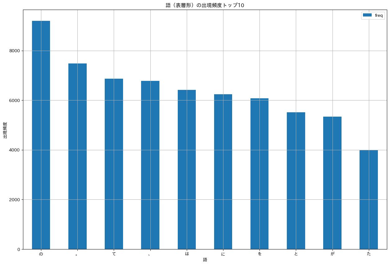
37. 頻度上位10語

出現頻度が高い10語とその出現頻度をグラフ（例えば棒グラフなど）で表示せよ.

import japanize_matplotlib
import matplotlib.pyplot as plt

offset = 10
fig, ax = plt.subplots(figsize=(20, 10))
df_surface_freqs[:offset].plot(kind='bar',
                               ax=ax,
                               title=f'語（表層形）の出現頻度トップ{offset}',
                               grid=True,
                               xlabel='語',
                               ylabel='出現頻度',
                               rot=0)
fig.show()

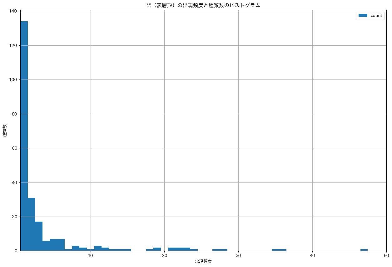
38. ヒストグラム

単語の出現頻度のヒストグラム（横軸に出現頻度, 縦軸に出現頻度をとる単語の種類数を棒グラフで表したもの）を描け.

import numpy as np

fig, ax = plt.subplots(figsize=(20, 10))
df_surface_freqs_agged = (df_surface_freqs['freq'].value_counts()
                                                  .reset_index()
                                                  .sort_values(by='freq'))
# Plot the first smallest 50 bins
offset = 50
bins = np.arange(offset) - 0.5
df_surface_freqs_agged.plot(x='freq',
                            y='count',
                            kind='hist',
                            bins=bins,
                            ax=ax,
                            title='語（表層形）の出現頻度と種類数のヒストグラム',
                            grid=True,
                            xlim=(0.5, offset),
                            xlabel='出現頻度',
                            ylabel='種類数',
                            rot=0)
fig.show()

39. Zipf の法則

単語の出現頻度順位を横軸, その出現頻度を縦軸として, 両対数グラフをプロットせよ.

fig, ax = plt.subplots(figsize=(20, 10))
df_surface_freqs.plot(kind='line',
                      ax=ax,
                      title='語（表層形）の出現頻度順位と出現頻度の対数プロット',
                      grid=True,
                      logx=True,
                      logy=True,
                      xticks=None,
                      xlabel='出現頻度順位（対数）',
                      ylabel='出現頻度(対数)',
                      rot=0)
fig.show()

References

Okazaki, N. (2015). 言語処理100本ノック 2015 [Natural Language Processing 100 Exercises 2015]. Retrieved from http://www.cl.ecei.tohoku.ac.jp/nlp100/
Okazaki, N. (2020). 言語処理100本ノック 2020 [Natural Language Processing 100 Exercises 2020]. Retrieved from https://nlp100.github.io/ja/

Share on

Twitter Facebook LinkedIn

Masaya Sato